Antibody clones

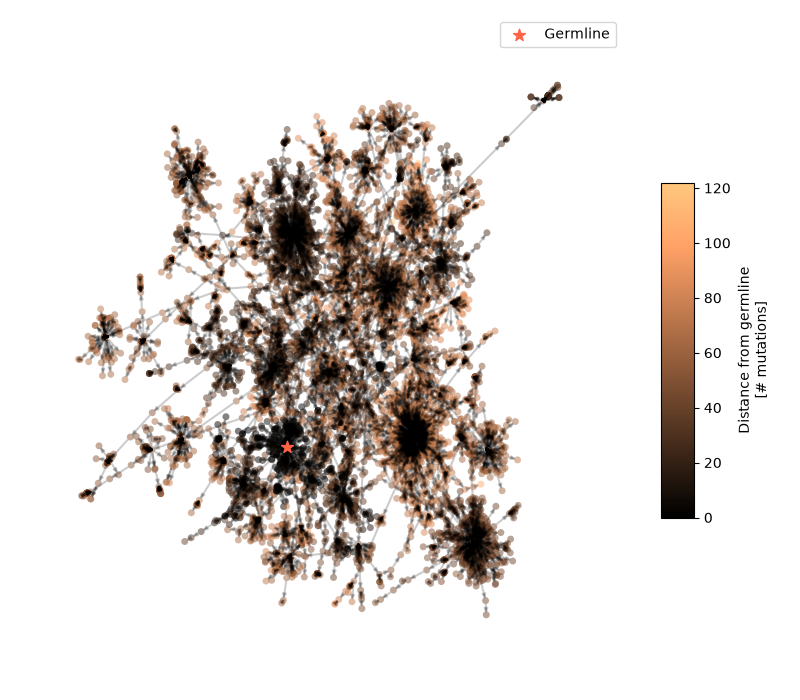
This example demonstrates how to visualise the antibodies of a large repertoire clone with iplotx.

This particular example uses igraph to load and process the network data, but you can also use networkx, the internal data structures of iplotx, or any other library you prefer.

Data source: Horns et al., Quake. et al. (2016): https://elifesciences.org/articles/16578.

import json
import igraph as ig
import pandas as pd
import matplotlib.pyplot as plt
import iplotx as ipx


# The original data format is a JSON file with source: {target1: distance1, target2: distance2, ...}
# We convert it into a DataFrame for igraph
with open("data/80201010000000001.mst") as handle:
    data = json.load(handle)
edge_data = {"source": [], "target": [], "distance": []}
for source, target_dict in data.items():
    for target, distance in target_dict.items():
        edge_data["source"].append(source)
        edge_data["target"].append(target)
        edge_data["distance"].append(distance)
edge_data = pd.DataFrame(edge_data)
edge_data["weight"] = 1 / edge_data["distance"]  # Invert distance to get some kind of weight

# NOTE: This particular format is a directed graph, from germline antibody to hypermutated antibody
g = ig.Graph.DataFrame(edge_data, directed=True, use_vids=False)

# Color nodes by distance from the germline antibody
germline = "8031,NA,germline,NA"
depths = {germline: 0.0}
to_visit = [germline]
while to_visit:
    node = to_visit.pop()
    for child, dist in data.get(node, {}).items():
        depths[child] = depths[node] + dist
        to_visit.append(child)
depth_max = max(depths.values())
colors = [depths[name] for name in g.vs["name"]]

# Compute bipartite layout
layout = g.layout_fruchterman_reingold()

fig, ax = plt.subplots(figsize=(8, 7))
artist = ipx.network(
    g,
    layout=layout,
    ax=ax,
    vertex_facecolor=colors,
    vertex_cmap=plt.cm.copper,
    vertex_alpha=0.5,
    vertex_size=5,
    edge_alpha=0.2,
    edge_arrow_width=2,
)[0]
fig.colorbar(
    artist.get_vertices(),
    ax=ax,
    label="Distance from germline\n[# mutations]",
    aspect=10,
    shrink=0.5,
)

# Label the germline antibody for clarity
coords_germline = layout[g.vs["name"].index(germline)]
ax.scatter([coords_germline[0]], [coords_germline[1]], color="tomato", s=80, marker="*", label="Germline")
ax.legend()
fig.tight_layout()

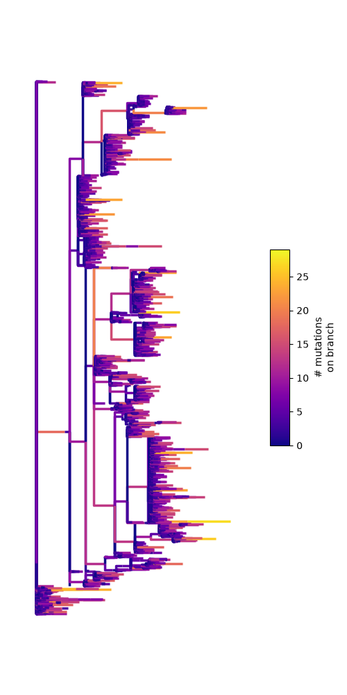
This graph turns out to be a tree, so we can revisualise the same data using a tree layout. As an example, we use our internal tree data structure, which is a glorified dictionary:

tree = {
    "children": [],
    "name": germline,
    "branch_length": 0.0,
}
to_visit = [(tree, germline)]
while to_visit:
    node, key = to_visit.pop()
    for child, dist in data.get(key, {}).items():
        child_node = {"children": [], "branch_length": dist, "name": child}
        node["children"].append(child_node)
        to_visit.append((child_node, child))
tree = ipx.ingest.providers.tree.simple.SimpleTree.from_dict(tree)

fig, ax = plt.subplots(figsize=(5, 10))
artist = ipx.tree(
    tree,
    ax=ax,
    edge_color="branch_length",
    edge_cmap=plt.cm.plasma,
)
fig.colorbar(
    artist.get_edges(),
    ax=ax,
    label="# mutations\non branch",
    fraction=0.07,
    aspect=10,
    shrink=0.5,
)
fig.tight_layout()