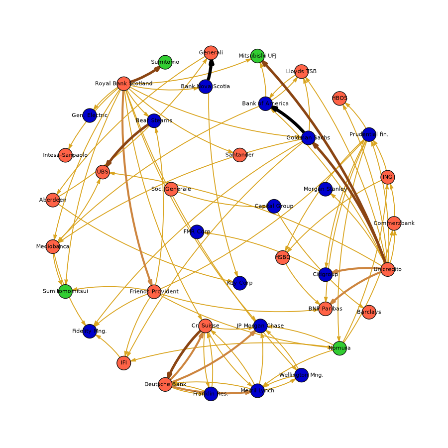
Financial network

This example demonstrates the use of iplotx to visualise financial relationships, mimicking a figure published in this paper: https://www.science.org/doi/10.1126/science.1173644.

from collections import defaultdict
import igraph as ig
import numpy as np
import pandas as pd
import matplotlib.pyplot as plt
import iplotx as ipx


# Circle nodes
g = ig.Graph(23, directed=True)
layout = g.layout_circle().coords
names = [
    "Commerzbank",
    "ING",
    "Prudential fin.",
    "HBOS",
    "Lloyds TSB",
    "Mitsubishi UFJ",
    "Generali",
    "Sumitomo",
    "Royal Bank Scotland",
    "Gen. Electric",
    "Intesa-Sanpaolo",
    "Aberdeen",
    "Mediobanca",
    "Sumitomomitsui",
    "Fidelity Mng.",
    "IFI",
    "Deutsche Bank",
    "Franklin Res.",
    "Merril Lynch",
    "Wellington Mng.",
    "Nomura",
    "Barclays",
    "Unicredito",
]

# Internal nodes
data_internal = [
    ["Bank Nova Scotia", -0.1, 0.8],
    ["Bear Stearns", -0.4, 0.6],
    ["UBS", -0.7, 0.3],
    ["Friends Provident", -0.4, -0.4],
    ["Cr. Suisse", -0.1, -0.6],
    ["Soc. Generale", -0.3, 0.2],
    ["FMR Corp", -0.15, -0.05],
    ["Bank of America", 0.25, 0.7],
    ["Santander", 0.1, 0.4],
    ["Citigroup", 0.6, -0.3],
    ["BNP Paribas", 0.6, -0.5],
    ["HSBC", 0.35, -0.2],
    ["JP Morgan Chase", 0.22, -0.6],
    ["Morgan Stanley", 0.6, 0.2],
    ["Goldman Sachs", 0.5, 0.5],
    ["Capital Group", 0.3, 0.1],
    ["Key Corp", 0.1, -0.35],
]
layout.extend([x[1:] for x in data_internal])
names.extend([x[0] for x in data_internal])
g.add_vertices(len(layout) - g.vcount())


g.vs["name"] = names

g.add_edges([
    (0, 1),
    (1, 2),
    (2, 3),
    (22, 0),
    (26, 2),
    (20, 0),
    (20, 1),
    (20, 18),
    (22, 2),
    (22, 3),
    (22, 4),
    (8, 5),
    (8, 9),
    (8, 10),
    (6, 11),
    (11, 6),
    (8, 12),
    (8, 13),
    (8, 23),
    (8, 24),
    (8, 27),
    (8, 31),
    (8, 37),
    (12, 13),
    (12, 14),
    (15, 14),
    (20, 15),
    (16, 17),
    (18, 16),
    (17, 16),
    (18, 19),
    (27, 35),
    (20, 35),
    (18, 35),
    (34, 33),
    (22, 36),
    (38, 21),
    (12, 25),
    (22, 25),
    (28, 38),
    (26, 13),
    (30, 5),
    (4, 30),
    (30, 4),
    (22, 30),
    (37, 4),
    (37, 12),
    (37, 14),
    (37, 15),
    (26, 15),
    (26, 14),
    (26, 24),
    (32, 29),
    (17, 27),
    (27, 17),
    (18, 27),
    (27, 18),
    (19, 18),
    (11, 39),
    (6, 39),
    (8, 35),
    (8, 19),
    (2, 34),
    (2, 32),
    (2, 33),
    (2, 20),
    (1, 34),
    (30, 12),
    (19, 35),
    (26, 20),
    (26, 33),
    # weight 2
    (8, 26),
    # weight 3
    (16, 27),
    (16, 35),
    (16, 18),
    (22, 32),
    (22, 33),
    # weight 4
    (8, 7),
    (27, 16),
    (24, 25),
    (22, 5),
    (22, 37),
    # weight 5
    (23, 6),
    (37, 30),
])

g.es["weight"] = 1
g.es[-2 -5 -5-1:]["weight"] = 3
g.es[-2 -5 -5:]["weight"] = 3
g.es[-2 -5:]["weight"] = 4
g.es[-2:]["weight"] = 5
edge_colord = {
    1: "goldenrod",
    2: "darkgoldenrod",
    3: "peru",
    4: "saddlebrown",
    5: "black",
}
g.es["color"] = [edge_colord[w] for w in g.es["weight"]]
g.es["linewidth"] = [0.5 + 0.8 * w for w in g.es["weight"]]

vertex_colors_inv = {
    "tomato": [
        "Commerzbank",
        "ING",
        "HBOS",
        "Lloyds TSB",
        "Royal Bank Scotland",
        "Deutsche Bank",
        "Barclays",
        "Unicredito",
        "Santander",
        "BNP Paribas",
        "Cr. Suisse",
        "IFI",
        "Friends Provident",
        "Soc. Generale",
        "Mediobanca",
        "BNP Paribas",
        "HSBC",
        "UBS",
        "Aberdeen",
        "Intesa-Sanpaolo",
        "Generali",
    ],
    "limegreen": [
        "Nomura",
        "Sumitomomitsui",
        "Sumitomo",
        "Mitsubishi UFJ",
    ],
}
vertex_colors = ["mediumblue" for x in g.vs["name"]]
for color, names in vertex_colors_inv.items():
    for name in names:
        try:
            idx = g.vs.find(name=name).index
        except ValueError:
            continue

        vertex_colors[idx] = color


fig, ax = plt.subplots(figsize=(9, 9))
ipx.network(
    g,
    layout,
    ax=ax,
    edge_color=g.es["color"],
    edge_curved=True,
    edge_tension=0.7,
    vertex_facecolor=vertex_colors,
    vertex_edgecolor="#111",
    vertex_zorder=3,
    vertex_labels=list(g.vs["name"]),
    vertex_label_color="black",
    vertex_label_size=8,
    edge_arrow_marker=")>",
    edge_arrow_width=4,
    edge_arrow_height=7,
    edge_linewidth=g.es["linewidth"],
)

fig.tight_layout()

plt.ion(); plt.show()