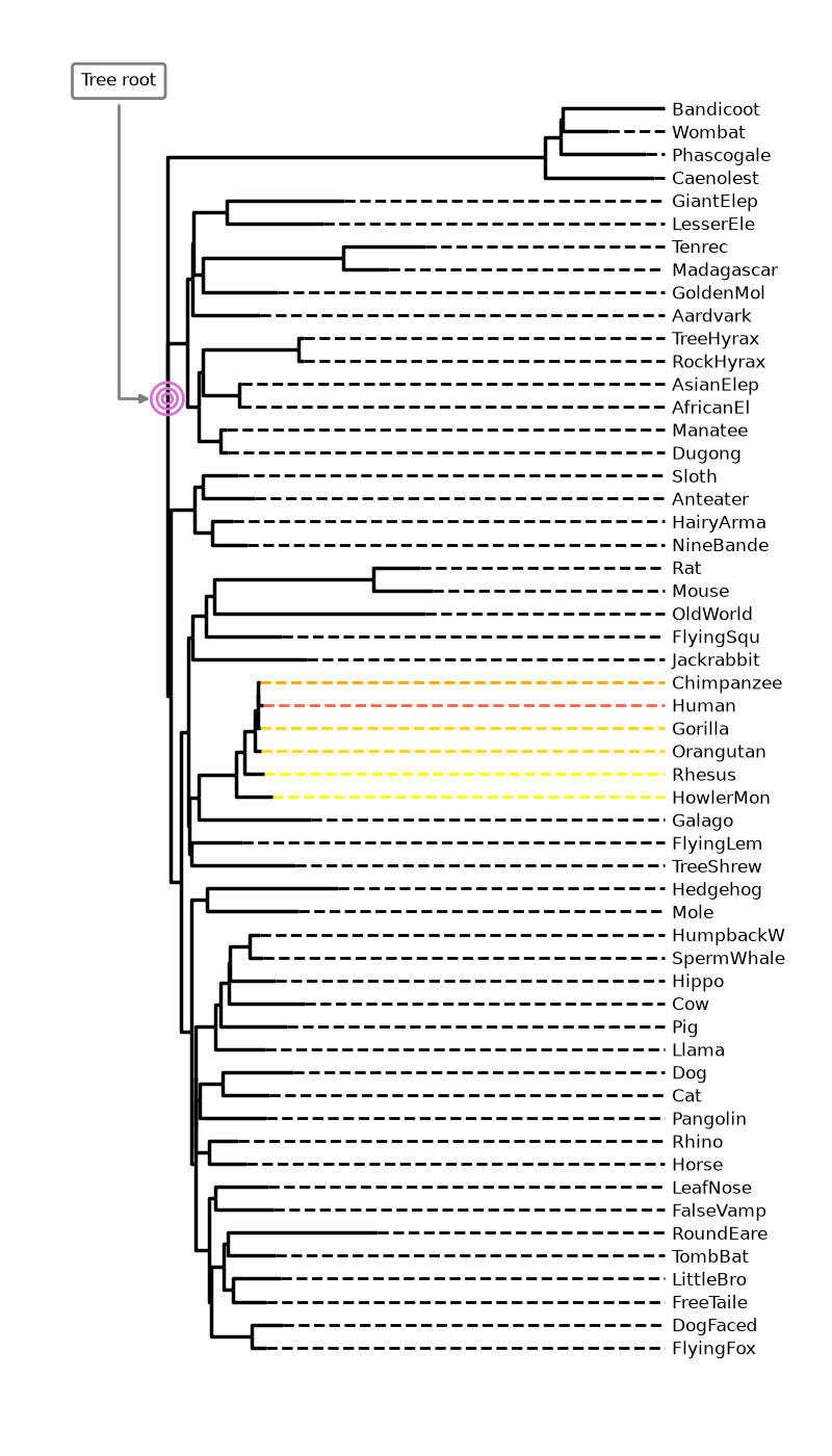
Animal phylogeny

This example from cogent3 shows how to use iplotx to visualise a phylogenetic tree of many animals.

It also shows how to combine iplotx trees with other matplotlib artists such as annotations and scatter plots.

from collections import defaultdict
import cogent3
import matplotlib.pyplot as plt
import iplotx as ipx

reader = cogent3.get_app("load_json")

ens_tree = reader("data/GN-tree.json")

# Customise the figure as you like
fig, ax = plt.subplots(figsize=(8, 14))

# Inject plot into the figure/axes
tree_artist = ipx.tree(
  ens_tree,
  layout="horizontal",
  ax=ax,
  leaf_labels=True,
  # Style options
  layout_angular=False,
  leaf_deep=True,
  margins=(0.2, 0),
  leafedge_color=defaultdict(lambda: "black", {
      "Human": "tomato",
      "Chimpanzee": "orange",
      "Orangutan": "gold",
      "Gorilla": "gold",
      "Rhesus": "yellow",
      "HowlerMon": "yellow",
  }),
  leafedge_linewidth=2,
)

# Add an annotation with an arrow towards the root
layout = tree_artist.get_layout().values
root_coords = layout[layout[:, 0] == 0][0]
ax.annotate(
    "Tree root",
    root_coords,
    (-0.1, 55),
    xycoords="data",
    textcoords="data",
    arrowprops=dict(
      color="grey",
      arrowstyle="-|>",
      shrinkA=4,
      shrinkB=12,
      linewidth=2,
      connectionstyle="angle",
    ),
    bbox=dict(
        boxstyle="round,rounding_size=0.2,pad=0.5",
        facecolor="white",
        edgecolor="grey",
        linewidth=2,
    ),
    fontsize=12,
)

# Also add concentric circles at the root
ax.scatter(
    [root_coords[0]] * 3,
    [root_coords[1]] * 3,
    s=[50, 200, 500],
    facecolor="none",
    edgecolor="orchid",
    linewidth=2,
)

# Ensure tight layout for minimal whitespace
fig.tight_layout()