Note
Go to the end to download the full example code.
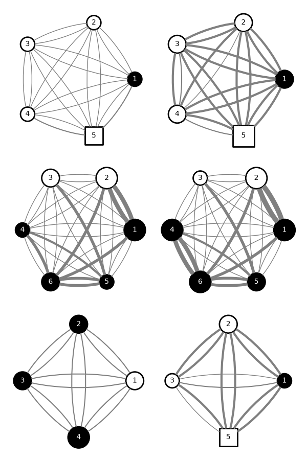
Foraging table#
This example visualises a table of foraging strategies, as found at https://doi.org/10.1111/1365-2656.13609.
Warning
The edge thicknesses are manually set to mimic the original figure a little, not derived from real data. This is just for illustration.
from collections import defaultdict
import numpy as np
import pandas as pd
import networkx as nx
import matplotlib.pyplot as plt
import iplotx as ipx


common_style = {
    "vertex": {
        "linewidth": 2,
        "edgecolor": "black",
    },
    "edge": {
        "color": "grey",
        "tension": 0.75,
        "curved": True,
        "arrow": {
            "width": 0,
        }
    }
}


# Create figure and subplots
fig, axs = plt.subplots(3, 2, figsize=(6, 9))

# Two examples with 5 nodes
g = nx.complete_graph(range(1, 6), nx.DiGraph)
layout = nx.circular_layout(g)
ipx.plot(
    g, layout, ax=axs[0, 0],
    vertex_labels=True,
    style=common_style,
    vertex_facecolor=["black"] + ["white"] * 4,
    vertex_label_color=["white"] + ["black"] * 4,
    vertex_marker=["o"] * 4 + ["s"],
    vertex_size=[20] * 4 + [25],
    edge_linewidth=defaultdict(lambda: 1, {(4, 5): 1.5, (5, 1): 1.5}),
)
ipx.plot(
    g, layout, ax=axs[0, 1],
    vertex_labels=True,
    style=common_style,
    vertex_facecolor=["black"] + ["white"] * 4,
    vertex_label_color=["white"] + ["black"] * 4,
    vertex_marker=["o"] * 4 + ["s"],
    vertex_size=[25] * 4 + [30],
    edge_linewidth=defaultdict(
        lambda: 3, {
            (4, 2): 1, (4, 3): 1.5, (4, 5): 1.5,
        },
    ),
)

# Two examples with 6 nodes
g = nx.complete_graph([1, 2, 3, 4, 6, 5], nx.DiGraph)
layout = nx.circular_layout(g)
ipx.plot(
    g, layout, ax=axs[1, 0],
    vertex_labels=True,
    style=common_style,
    vertex_facecolor=["black"] + ["white"] * 2 + ["black"] * 3,
    vertex_label_color=["white"] + ["black"] * 2 + ["white"] * 3,
    vertex_size=[30] * 2 + [25, 20]  * 2,
    edge_linewidth=defaultdict(
        lambda: 1, {
            (1, 2): 6, (2, 1): 6, (6, 2): 4, (6, 4): 4, (6, 1): 4, (6, 5): 4, (5, 6): 4, (5, 3): 4, (5, 4): 3,
        },
    ),
)
ipx.plot(
    g, layout, ax=axs[1, 1],
    vertex_labels=True,
    style=common_style,
    vertex_facecolor=["black"] + ["white"] * 2 + ["black"] * 3,
    vertex_label_color=["white"] + ["black"] * 2 + ["white"] * 3,
    vertex_size=[30] * 2 + [20] + [30] * 2 + [25],
    edge_linewidth=defaultdict(
        lambda: 1, {
            (1, 2): 7, (2, 1): 7, (6, 2): 4, (6, 4): 6, (4, 6): 6, (6, 1): 4, (6, 5): 4, (5, 6): 4, (5, 3): 4, (5, 4): 3,
        },
    ),
)

# Two examples with 4 nodes
g = nx.complete_graph(range(1, 5), nx.DiGraph)
layout = nx.circular_layout(g)
ipx.plot(
    g, layout, ax=axs[2, 0],
    vertex_labels=True,
    style=common_style,
    vertex_facecolor=["white"] + ["black"] * 3,
    vertex_label_color=["black"] + ["white"] * 3,
    vertex_size=[25] * 3 + [30],
)

g = nx.complete_graph([1, 2, 3, 5], nx.DiGraph)
layout = nx.circular_layout(g)
ipx.plot(
    g, layout, ax=axs[2, 1],
    vertex_labels=True,
    style=common_style,
    vertex_facecolor=["black"] + ["white"] * 3,
    vertex_label_color=["white"] + ["black"] * 3,
    vertex_size=[20, 25] * 2,
    vertex_marker=["o"] * 3 + ["s"],
    edge_linewidth=defaultdict(
        lambda: 3, {
            (1, 3): 1, (3, 1): 1.5, (3, 5): 1,
        },
    ),
)


fig.tight_layout()
Total running time of the script: (0 minutes 0.319 seconds)