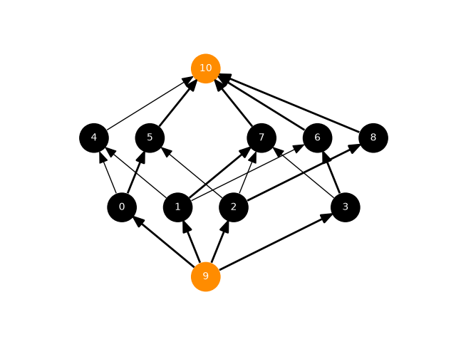
Maximum Bipartite Matching by Maximum Flow

This example from igraph presents how to visualise bipartite matching using maximum flow, with edge linewidth and vertex facecolor styling.

import igraph as ig
import iplotx as ipx

# We start by creating the bipartite directed graph.
g = ig.Graph(
    9,
    [(0, 4), (0, 5), (1, 4), (1, 6), (1, 7), (2, 5), (2, 7), (2, 8), (3, 6), (3, 7)],
    directed=True,
)

# We assign:
#  - nodes 0-3 to one side
#  - nodes 4-8 to the other side
g.vs[range(4)]["type"] = True
g.vs[range(4, 9)]["type"] = False

# Then we add a source (vertex 9) and a sink (vertex 10)
g.add_vertices(2)
g.add_edges([(9, 0), (9, 1), (9, 2), (9, 3)])  # connect source to one side
g.add_edges([(4, 10), (5, 10), (6, 10), (7, 10), (8, 10)])  # ... and sinks to the other

# Compute maximum flow
flow = g.maxflow(9, 10)

# To achieve a pleasant visual effect, we set the positions of source and sink
# manually:
layout = g.layout_bipartite()
layout[9] = (2, -1)
layout[10] = (2, 2)

ipx.network(
    g,
    layout=layout,
    vertex_labels=True,
    style={
        "vertex": {
            "size": 30,
            "facecolor": ["black" if i < 9 else "darkorange" for i in range(11)],
        },
        "edge": {
            "linewidth": [1.0 + flow.flow[i] for i in range(g.ecount())],
        },
    },
)

[<iplotx.network.NetworkArtist object at 0x7af390c26e90>]

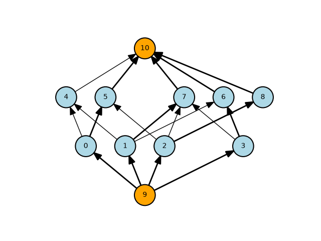
If you want to have dark labels on light background, you can set the vertex style accordingly, perhaps with pronounced vertex borders to increase constrast:

ipx.network(
    g,
    layout=layout,
    vertex_labels=True,
    style={
        "vertex": {
            "size": 30,
            "facecolor": ["lightblue" if i < 9 else "orange" for i in range(11)],
            "edgecolor": "black",
            "linewidth": 1.5,
            "label": {
                "color": "black",
            },
        },
        "edge": {
            "linewidth": [1.0 + flow.flow[i] for i in range(g.ecount())],
        },
    },
)  #

[<iplotx.network.NetworkArtist object at 0x7af38fdb6710>]